Ingo's Blog

Open and plot of all files in a register ( German ) This plot is about to open and plot all files in a register with Matlab. First of all, all files with the format *.txt are opend and saved in files. files = dir('*.csv'); For value = 2 just every second file is saved. for i = 1:1:length(files)/value     fid3{i}=files(i).name; end To sort these files by name you need to download "natsortfiles" from Matlab-Exchang: fid3 = natsortfiles(fid3) for i = 1:value:length(files)      fid = fopen(fid3{i});     daten = textscan(fid,'%f %f','delimiter',',','headerlines',0');     q1(:,i/value) = daten(1);     q2(:,i/value) = daten(2); end fclose(fid); In "textscan" with 'headlines',0 is the amount of rows are defined which are delited from the text file. The files from coulomn 1 are saved in q1 and from coulomn 2 are saved in q2. Furthermore the files are opened and saved in a matrix and in a defin...

Colorspectra with Matlab ( German ) This post is about a Matlab-function, to generate colorspectras for multiple plots. Therefor you can change the colorsweep in different way. This is the function ( Download ): function [CoolSpec] = ColSpec(a,q,value,start) On can define with "a" the amount of different colors in the area between red over yellow to green to blue to pink and further to red. q displays the q'th value of the generated spectra. With "value" the width of the spectra is described wherefor value>1 decreases the spectrawidth. "start" is the startingvalue for the color. Therefor red is (start = 0), yellow (start = 0.5), green(start = 1), brightblue (start = 1.5-2), darkblue(start = 2.5) and pink (start = 3) and the again red and so on. With "m" and "k" is the darkness for values smaller 1. "inv" inverte the colorspec for values unequal zero from blue over green to red. Here a different parameters sh...

Optical composition with Matlab ( German ) This post is about the representation of optical compositions existing of lenses, mirror and other optics. Therefore I programmed a few functions which are described below ( MATLAB files ): opticlense(x,y,deg,thick,dx,dy,color) opticbeamsplitter(x,y,deg, thick,dx,dy,color) opticbikonvex( x,y,deg,thick,dx,dy,color)  opticdistance(x1,y1,x2,y2,string,len,thick,color) opticline(x,y,deg,len,thick,color) opticmirror(x,y,deg,style,thick,color,len) opticslit(x,y,deg,thick,color,len) Therefor x and y are the positions of the optical element. The optics are positioned scaled. deg is the angle of the inclination and dx , dy and len the length in x, y direction. color is the color and thick the thickness of the line. In opticdistance x1 , y1 are initial values and x2 , y2 the final valueswhere string stands for the name (for example the distance). In opticmirror style as the value 0 returns a normal mirror and for the value 1 a das...

General: ( German ) A Theremin is an electric musical instrument, which is regulated by two resonant circuits. One resonant circuit is connected to an antenna. Through changing the distance between you and the antenna you change the frequency of the resonant circuit. At least you can hear the difference between both circuits. Composition: You need these components and the following circuit: OPV TL071 x2 LM386 x1 Capacitors: 100 nF x2 220 nF x2 47 pF x2 47 nF x1 100 pF x1 10 nF x1 Elko 220 u x3 Resistors: 100 k  x4 22 k x4 47 k x2 10 x1 Potientiometer 100k x1 10k x2 Others: Diode 1N4007 1 BAT42 2 Antenna Speaker To supply the Theremin with electricity ja can use two 9V-batteries in series. With power supplies you have to be careful because they have to be grounded with this plug . Left you see my composition at the stickboard additional with on-off-plug and speaker connection. Important is to use short wires to reduce the disturbance of the reso...

Cone/Arrow in 3D To plot a cone or arrow in 3D you can use this function: function arrow3D(startVec, stopVec, varargin) The startVec is the beginning of the 3D cone and the stopVec the end of the cone. Ypi can use the optional arguments as 'Color','Thickness','Length' to customize your cone. Source code : function arrow3D(startVec,stopVec,varargin) % Input arguments: % startVec ... input vector of the beginning of the point in [x,y,z] % stopVec ... input vector of the ending of the point in [x,y,z] % % Optional input argument (varargin): % 'Color',color ... define the color of the arrow/point % 'Thickness',thick ... thickness of the arrow % 'Length',length ... Length of the arrow % 'Axes',ax ... Input axes     if isempty(varargin)         varargin{1} = '';     end          [x] = startVec(1);      [y] = startVec(2);      [z] = startVec(3);      x2 = stopVec(1);   ...

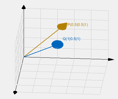
Points and Vectors in 3D-Plots (German) This matlabfunction creates vectors and points for the previous post in the 3D cartesian coordinate system. function punkt3D(x1,y1,z1,x2,y2,z2,sign,name,color,dx,dy,dz,true) Therefor "startVec" are the initial values of the vector and "stopVec" the final values. You need the function ( Cone/Arrow ) and  ( Grid3D ). The optional arguments are shown below. For example you can use it as: figure;hold on;axis off; grid3D([0,0,0], [1,1,1], 'Amount', [4,4,4], 'Axes', gca, 'MinorGrid','Arrow','AxTicks',[{['']},{['']},{['']}],...     'AxLabels',["";"";""]); P = [0.5,0.5,1]; Q = [1,0.5,1]; point3D([0,0,0],P,'Marker','arrow','Label','P(0.5|0.5|1)','Color',[0.7 0.5 0]); point3D([0,0,0],Q,'Marker','arrow','Label','Q(1|0.5|1)','Color',[0.0 0.4 0.74],'D...

3D Grid/Gitter (German) This plot is to generate a 3D-lattice for Matlab. In dependence of a few arguments you can use this function to plot easy 3D vectors and flats as seen in function grid3D(startVec,stopVec,varargin) With the variables startVec and stopVec you can specify the direction of the Cartesian grid that will be plotted. Optional arguments like color, thickness can be applied as described in the function. figure;hold on;axis off; grid3D([0,0,0], [1,1,1], 'Amount', [4,4,4], 'Axes', gca, 'MinorGrid','Arrow' ); P = [0.5,0.5,1]; Q = [1,0.5,1]; point3D([0,0,0],P,'Marker','arrow','Label','P(0.5|0.5|1)','Color',[0.7 0.5 0]); point3D([0,0,0],Q,'Marker','arrow','Label','Q(1|0.5|1)','Color',[0.0 0.4 0.74],'Deviation',[0,0,0.1]); In addition, the grid can also be rotated. For example, a projection of two coordinate systems can be displayed: f igure;hold on;axis o...