Ingo's Blog

General: ( German ) A Theremin is an electric musical instrument, which is regulated by two resonant circuits. One resonant circuit is connected to an antenna. Through changing the distance between you and the antenna you change the frequency of the resonant circuit. At least you can hear the difference between both circuits. Composition: You need these components and the following circuit: OPV TL071 x2 LM386 x1 Capacitors: 100 nF x2 220 nF x2 47 pF x2 47 nF x1 100 pF x1 10 nF x1 Elko 220 u x3 Resistors: 100 k  x4 22 k x4 47 k x2 10 x1 Potientiometer 100k x1 10k x2 Others: Diode 1N4007 1 BAT42 2 Antenna Speaker To supply the Theremin with electricity ja can use two 9V-batteries in series. With power supplies you have to be careful because they have to be grounded with this plug . Left you see my composition at the stickboard additional with on-off-plug and speaker connection. Important is to use short wires to reduce the disturbance of the resonant

Cone/Arrow in 3D To plot a cone or arrow in 3D you can use this function: function arrow3D(startVec, stopVec, varargin) The startVec is the beginning of the 3D cone and the stopVec the end of the cone. Ypi can use the optional arguments as 'Color','Thickness','Length' to customize your cone. Source code : function arrow3D(startVec,stopVec,varargin) % Input arguments: % startVec ... input vector of the beginning of the point in [x,y,z] % stopVec ... input vector of the ending of the point in [x,y,z] % % Optional input argument (varargin): % 'Color',color ... define the color of the arrow/point % 'Thickness',thick ... thickness of the arrow % 'Length',length ... Length of the arrow % 'Axes',ax ... Input axes     if isempty(varargin)         varargin{1} = '';     end          [x] = startVec(1);      [y] = startVec(2);      [z] = startVec(3);      x2 = stopVec(1);     y2 = stopVec(2);     z2 = stopVec(3);          [logi

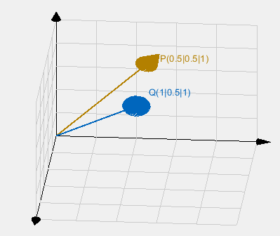
Points and Vectors in 3D-Plots (German) This matlabfunction creates vectors and points for the previous post in the 3D cartesian coordinate system. function punkt3D(x1,y1,z1,x2,y2,z2,sign,name,color,dx,dy,dz,true) Therefor "startVec" are the initial values of the vector and "stopVec" the final values. You need the function ( Cone/Arrow ) and  ( Grid3D ). The optional arguments are shown below. For example you can use it as: figure;hold on;axis off; grid3D([0,0,0], [1,1,1], 'Amount', [4,4,4], 'Axes', gca, 'MinorGrid','Arrow','AxTicks',[{['']},{['']},{['']}],...     'AxLabels',["";"";""]); P = [0.5,0.5,1]; Q = [1,0.5,1]; point3D([0,0,0],P,'Marker','arrow','Label','P(0.5|0.5|1)','Color',[0.7 0.5 0]); point3D([0,0,0],Q,'Marker','arrow','Label','Q(1|0.5|1)','Color',[0.0 0.4 0.74],'D

3D Grid/Gitter (German) This plot is to generate a 3D-lattice for Matlab. In dependence of a few arguments you can use this function to plot easy 3D vectors and flats as seen in function grid3D(startVec,stopVec,varargin) With the variables startVec and stopVec you can specify the direction of the Cartesian grid that will be plotted. Optional arguments like color, thickness can be applied as described in the function. figure;hold on;axis off; grid3D([0,0,0], [1,1,1], 'Amount', [4,4,4], 'Axes', gca, 'MinorGrid','Arrow' ); P = [0.5,0.5,1]; Q = [1,0.5,1]; point3D([0,0,0],P,'Marker','arrow','Label','P(0.5|0.5|1)','Color',[0.7 0.5 0]); point3D([0,0,0],Q,'Marker','arrow','Label','Q(1|0.5|1)','Color',[0.0 0.4 0.74],'Deviation',[0,0,0.1]); In addition, the grid can also be rotated. For example, a projection of two coordinate systems can be displayed: f igure;hold on;axis o

Polar-Plots (German) If you use Matlabtikz and you want to create a polar plot, latex does not plot the axis. That's why i wrote this polargrid function. polartikzlabel(angleticks,abs,ticks,absdeg,anglestr,absstr,round1) Therefor "angleticks" the amount of subdivisions of the angle, "abs" the radius, "ticks" the amunt of the subdivisions of the radial scale, "absdeg" the angle of the radialtext. "anglestr" is the text of the anglescale "absstr" is the text of the radial scale. "round1" is the amount of internal decimal places. Dies kann wie folgt aussehen: polartikzlabel(5,1,6,40,'angle','radial',3) Source code : function polargrid(angleticks,abs,ticks,absdeg,anglestr,absstr,round1) %angleticks set the number of ticks in equidistant angles. %abs set the radius of the polarplot. %ticks set the number of ticks in equidistant radialskale. %absdeg set the degree of the radialaxis

Matlabplots in Latex (MATLABTIKZ) (German) If you use Latex and want to include a graphic in scalable size and the font and style of your latex document, you need MATLABTIKZ. The implement is as follows: h(1) = figure(1); ... matlab2tikz('runge.tikz', 'height', '\figureheight', 'width','\figurewidth', 'figurehandle', h(1)); The packages that are needed in latex: \usepackage{pgfplots} \usepackage{grffile} \pgfplotsset{compat=newest} \usetikzlibrary{plotmarks} \usepgfplotslibrary{polar} \usepgfplotslibrary{patchplots} To include pictures: \begin{figure}[H] \newlength\figureheight\setlength\figureheight{5.5cm} \newlength\figurewidth\setlength\figurewidth{0.65\textwidth} \input{runge.tikz} \captionof{figure}{Runge-Kutta-Verfahren 2. Ordnung} \end{figure} On this Page it's written to ad --shell-escape to the command pdflatex       pdflatex.exe -synctex=1 -interaction=nonstopmode

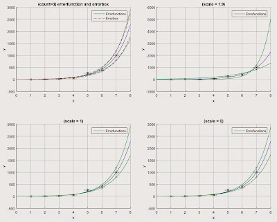
Supplement to errorlines with Matlab Exponential Fitting (German) This plot is about the previous post with exponential behavior of the form "b*(exp(a*x)". The structur is the same as in "Errorlines" but it has one further input value. function [smax,smin,rmax,rmin] = errexpfunc(x,y,xerr,yerr, count,scale) "Scale" is the position of the interception auf the two functions in dependence of the x-values. The interception is fpr "scale = 0" at the first x-value, "scale = 2" at the last x-value and "scale = 1" in the middle. source code: function [smax,smin,rmax,rmin] = errexpfunc(x,y,xerr,yerr, count,scale) %This is a function to plot a maximal and minimal errorline with given %errors 'xerr' and 'yerr'. It also can create the box around the mesured %values to see in which area the errorlines are plotted. %For count 1 it plots just the errorline. For count 2 it plots the box and %count 3 it pl

Messwertfilter: Verfahren: (German) The Matlab function is used to exclude measurevalues with big variation in linear relation and to fit through the remaining values. This works equal to Matlab:errorlines . Therefor you can change the variation to exclude more or less measure values. If there is a measure value with oversized value the function excludes it and fit again a linear relation how in this figure seen:   In red the errorbox and excludes measure value. Implementation: This function is called in Matlab with:"[x,y,xerr,yerr,xaus,yaus,xerraus,yerraus] = filterfunc(x, y, xerr, yerr, scale, count)". Therefor "xaus,yaus" are the filtered x- and y-values. "x,y,xerr,yerr" are the values you measured.  "Scale" determines how the variation. For (scale = 1) the function takes "yerr". As follows here are several approaches of this function: If (count = 1) the function plots a errorbox. Source code: function [x,y,x

The methode: (German) This post is about plotting errorlines for example for university journals. The methode is to fit a maximal and a minimal line through the y-values an whose error. As shown in the graph it yield a box. The errorlines are connection of the edges diagonal. The function "[varargout] = errlinefunc(x, y,xerr,yerr, varargin)" plots the error lines in blue. The color can be changed using ('LineColor',[0.5 0.5 0]) for example to orange or the line width ca be changed by ('LineWidth',2). The option 'Fit' plots in greeb ('FitColor') the linear fit through the data set. The option 'Plot' depicts the x and y with corresponding errorbars in black ('PlotColor'). 'Box' shows im black ('BoxColor') the borders of the errorlines. 'Legend' writes a legend with options 'Location','NorthEast' and similare and 'LegendNames',{['1','2','3']} changes the