Ingo's Blog

Segmentation Growing ( German ) This post is about a methode of segmentation where a region is defined (seed) . In this seed the standard deviation and the mean is calculated and with a factor f it is weigthed. Pixel which are in the neighborhood of the seed are added to the seed if their value is in the boundary defined by the standard deviation, mean value and weighting factor f. This is done iterative as long as no more pixel is added to the seed. Then the object is segmented. function [region, area, seed, sx1, sx2, sy1, sy2] = Segmentation_Growing(img,sx1,sx2,sy1,sy2,f): This function needs an image as an imput. If there is no other input value one can choose with to cursors the starting point sx1, sy1, the left upper corner, and the end point sx2, sy2, the right lower corner. Otherwise one can define the s-value as one wants. If one uses cursors, one can use the second input argument for defining the factor f. This factor describes the weigthing and is in an area bigger equa

The Dijkstra Methode - large neighborhood ( German )This is an update for the Dijkstra methode from the post before, where it uses now a larger neighborhood. It needs a bit longer but the probability to find the shortest path of many possible paths in the neighborhood is much higher. Here the comparing picture to Dijkstra Methode . Here one can download the following code on MathWorks: Source Code Dijkstra: function [path, prev, unvis, distance, start, target] = Dijkstra_Methode(Matrix, start, target) %Matrix is the incoming image %start is the start point in a vector [a,b] where a is the column and b the %row %target is the end point similare to start %path is the matrix with ones excepted at the position of the path where it is 0 %prev are also the previous visited pixels where the algorithm took the %wrong way %unvis are all unvisited pixels %distance is the distance or weight of the pixels %open the image and you can choose with the cursor the start %and end point if you d

The Dijkstra Methode ( German ) In this post i show you with Matlab how to calculate the shortest path on a gradient images with d´the dijkstra methode i wrote. I take an image as an input and convert it to an double and calculate the gradient [G,Gdir] = imgradient(img,'sobel'); and I use my function Dijkstra(G,p,q) : THis function needs a image as double G , a start value p and the target q , where the first entry of the oints is the column and the second the row. This methode sets all distances to infinity except the at the start value is zero obviously. All unvisited pixels have the value 1. The algortihm continous as long as the target is an unvisible pixel. For all neighborhood pixels the weights are calculated with the function [weight] = localedgewidth(G,p,q) ,where the value of the neightbor pixel is substract by the maximum of the matrix and devided by the difference of maximal and minimal value of the matrix G and multiplied with the distance to the neighbor pi

Generating a GUI interfaces ( German ) In this post I show you how to generate a GUI interface with Matlab with buttons, checkboxes ... There one has to write "guide" in the console of Matlab and a window opens where you can create a new interface or load an old one. Now an editor opens where you easily can put the objects you want in. You can safe it an then the Matlab code is generated. To program it, it is important that you relate to each object an "tag". This you can do by double click on the object. An Inspector opens where you can edit it an other things like the "value", "name" or the design: Now one can push the green arrow to generate the code where you can define your functions: Programmieren des GUI interfaces The button can be programmed in the code under "function pushbutton1_Callback(hObject, eventdata, handles)". In this case the program generates a coil in "axes1" in dependence of the value in

Open and plot of all files in a register ( German ) This plot is about to open and plot all files in a register with Matlab. First of all, all files with the format *.txt are opend and saved in files. files = dir('*.csv'); For value = 2 just every second file is saved. for i = 1:1:length(files)/value     fid3{i}=files(i).name; end To sort these files by name you need to download "natsortfiles" from Matlab-Exchang: fid3 = natsortfiles(fid3) for i = 1:value:length(files)      fid = fopen(fid3{i});     daten = textscan(fid,'%f %f','delimiter',',','headerlines',0');     q1(:,i/value) = daten(1);     q2(:,i/value) = daten(2); end fclose(fid); In "textscan" with 'headlines',0 is the amount of rows are defined which are delited from the text file. The files from coulomn 1 are saved in q1 and from coulomn 2 are saved in q2. Furthermore the files are opened and saved in a matrix and in a defined area

Colorspectra with Matlab ( German ) This post is about a Matlab-function, to generate colorspectras for multiple plots. Therefor you can change the colorsweep in different way. This is the function ( Download ): function [CoolSpec] = ColSpec(a,q,value,start) On can define with "a" the amount of different colors in the area between red over yellow to green to blue to pink and further to red. q displays the q'th value of the generated spectra. With "value" the width of the spectra is described wherefor value>1 decreases the spectrawidth. "start" is the startingvalue for the color. Therefor red is (start = 0), yellow (start = 0.5), green(start = 1), brightblue (start = 1.5-2), darkblue(start = 2.5) and pink (start = 3) and the again red and so on. With "m" and "k" is the darkness for values smaller 1. "inv" inverte the colorspec for values unequal zero from blue over green to red. Here a different parameters sh

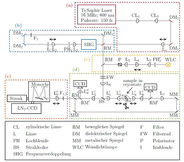
Optical composition with Matlab ( German ) This post is about the representation of optical compositions existing of lenses, mirror and other optics. Therefore I programmed a few functions which are described below ( MATLAB files ): opticlense(x,y,deg,thick,dx,dy,color) opticbeamsplitter(x,y,deg, thick,dx,dy,color) opticbikonvex( x,y,deg,thick,dx,dy,color)  opticdistance(x1,y1,x2,y2,string,len,thick,color) opticline(x,y,deg,len,thick,color) opticmirror(x,y,deg,style,thick,color,len) opticslit(x,y,deg,thick,color,len) Therefor x and y are the positions of the optical element. The optics are positioned scaled. deg is the angle of the inclination and dx , dy and len the length in x, y direction. color is the color and thick the thickness of the line. In opticdistance x1 , y1 are initial values and x2 , y2 the final valueswhere string stands for the name (for example the distance). In opticmirror style as the value 0 returns a normal mirror and for the value 1 a dashed

General: ( German ) A Theremin is an electric musical instrument, which is regulated by two resonant circuits. One resonant circuit is connected to an antenna. Through changing the distance between you and the antenna you change the frequency of the resonant circuit. At least you can hear the difference between both circuits. Composition: You need these components and the following circuit: OPV TL071 x2 LM386 x1 Capacitors: 100 nF x2 220 nF x2 47 pF x2 47 nF x1 100 pF x1 10 nF x1 Elko 220 u x3 Resistors: 100 k  x4 22 k x4 47 k x2 10 x1 Potientiometer 100k x1 10k x2 Others: Diode 1N4007 1 BAT42 2 Antenna Speaker To supply the Theremin with electricity ja can use two 9V-batteries in series. With power supplies you have to be careful because they have to be grounded with this plug . Left you see my composition at the stickboard additional with on-off-plug and speaker connection. Important is to use short wires to reduce the disturbance of the resonant

Cone/Arrow in 3D To plot a cone or arrow in 3D you can use this function: function arrow3D(startVec, stopVec, varargin) The startVec is the beginning of the 3D cone and the stopVec the end of the cone. Ypi can use the optional arguments as 'Color','Thickness','Length' to customize your cone. Source code : function arrow3D(startVec,stopVec,varargin) % Input arguments: % startVec ... input vector of the beginning of the point in [x,y,z] % stopVec ... input vector of the ending of the point in [x,y,z] % % Optional input argument (varargin): % 'Color',color ... define the color of the arrow/point % 'Thickness',thick ... thickness of the arrow % 'Length',length ... Length of the arrow % 'Axes',ax ... Input axes     if isempty(varargin)         varargin{1} = '';     end          [x] = startVec(1);      [y] = startVec(2);      [z] = startVec(3);      x2 = stopVec(1);     y2 = stopVec(2);     z2 = stopVec(3);          [logi

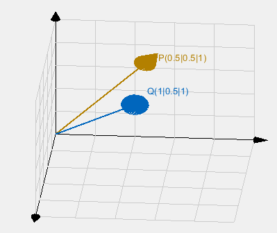
Points and Vectors in 3D-Plots (German) This matlabfunction creates vectors and points for the previous post in the 3D cartesian coordinate system. function punkt3D(x1,y1,z1,x2,y2,z2,sign,name,color,dx,dy,dz,true) Therefor "startVec" are the initial values of the vector and "stopVec" the final values. You need the function ( Cone/Arrow ) and  ( Grid3D ). The optional arguments are shown below. For example you can use it as: figure;hold on;axis off; grid3D([0,0,0], [1,1,1], 'Amount', [4,4,4], 'Axes', gca, 'MinorGrid','Arrow','AxTicks',[{['']},{['']},{['']}],...     'AxLabels',["";"";""]); P = [0.5,0.5,1]; Q = [1,0.5,1]; point3D([0,0,0],P,'Marker','arrow','Label','P(0.5|0.5|1)','Color',[0.7 0.5 0]); point3D([0,0,0],Q,'Marker','arrow','Label','Q(1|0.5|1)','Color',[0.0 0.4 0.74],'D

3D Grid/Gitter (German) This plot is to generate a 3D-lattice for Matlab. In dependence of a few arguments you can use this function to plot easy 3D vectors and flats as seen in function grid3D(startVec,stopVec,varargin) With the variables startVec and stopVec you can specify the direction of the Cartesian grid that will be plotted. Optional arguments like color, thickness can be applied as described in the function. figure;hold on;axis off; grid3D([0,0,0], [1,1,1], 'Amount', [4,4,4], 'Axes', gca, 'MinorGrid','Arrow' ); P = [0.5,0.5,1]; Q = [1,0.5,1]; point3D([0,0,0],P,'Marker','arrow','Label','P(0.5|0.5|1)','Color',[0.7 0.5 0]); point3D([0,0,0],Q,'Marker','arrow','Label','Q(1|0.5|1)','Color',[0.0 0.4 0.74],'Deviation',[0,0,0.1]); In addition, the grid can also be rotated. For example, a projection of two coordinate systems can be displayed: f igure;hold on;axis o